这是TensorBoard笔记的第二篇，讲述的是如何令TensorBoard展示外界已有的图片和Tensor。

我们可以利用TensorBoard展示图片类数据，或者通过tf.summary将张量类数据转化成图片。下面是对Fashion-MNIST数据集中部分图片的可视化：

可视化单个图片

import tensorflow as tf
from tensorflow import keras

fashion_mnist = keras.datasets.fashion_mnist
(train_images, train_labels), (test_images, test_labels) = \
    fashion_mnist.load_data()

数据集中每个图像的形状都是2阶张量形状（28、28），分别表示高度和宽度

但是， tf.summary.image()期望包含(batch_size, height, width, channels)的4级张量。因此，张量需要重塑。

img = np.reshape(train_images[0], (-1, 28, 28, 1))

使用tf.summary.image将其转化为tensor，并利用TensorBoard可视化：

 # Clear out any prior log data.
!rm -rf logs

# Sets up a timestamped log directory.
logdir = "logs/train_data/" + datetime.now().strftime("%Y%m%d-%H%M%S")
# Creates a file writer for the log directory.
file_writer = tf.summary.create_file_writer(logdir)

# Using the file writer, log the reshaped image.
with file_writer.as_default():
  tf.summary.image("Training data", img, step=0)

转化后的图片被tf.summary.create_file_writer输出到logdir里面了。使用TensorBoard看看：

%tensorboard --logdir logs/train_data

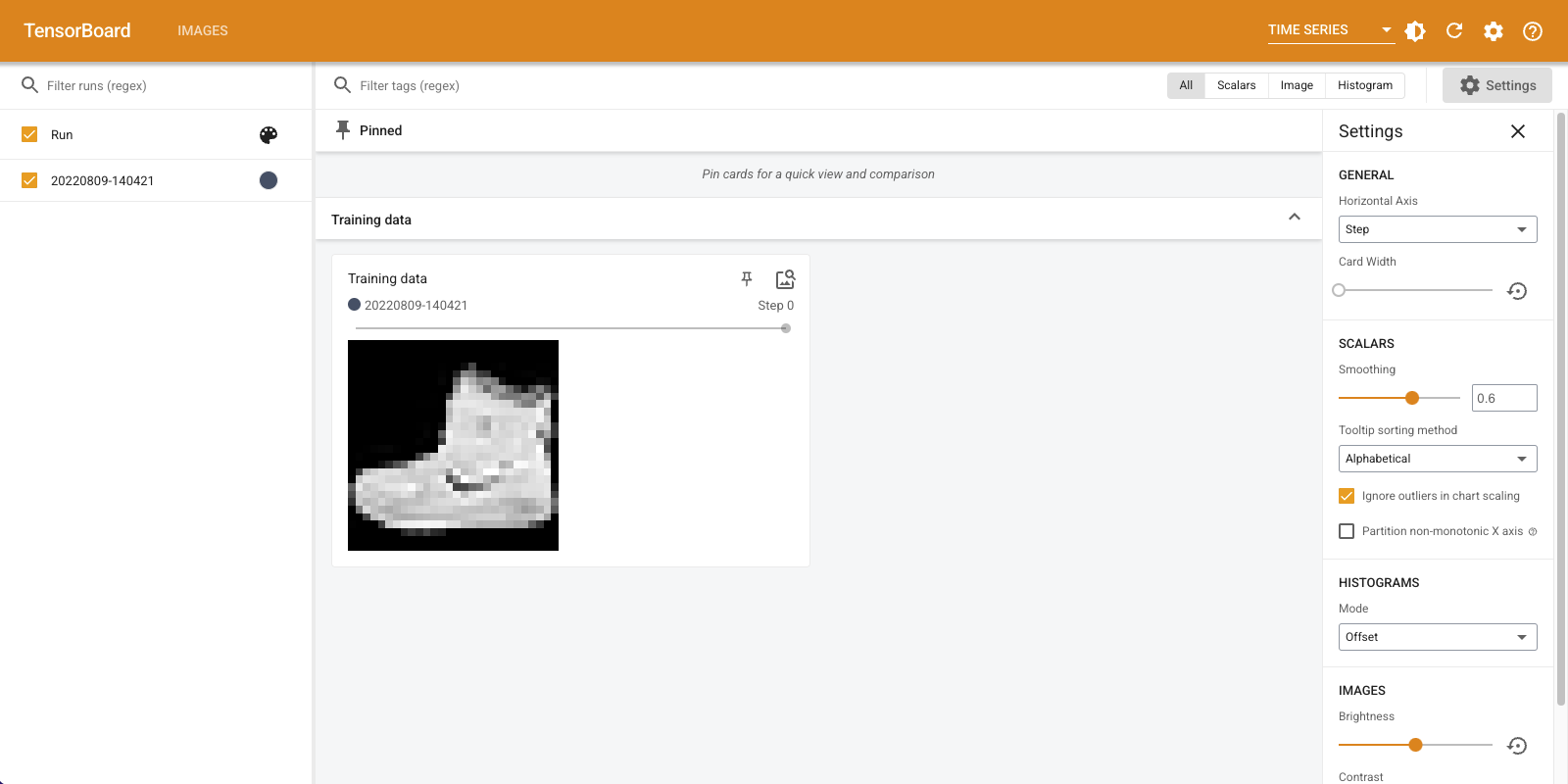
加载的过程可能有点慢，注意留足够的内存以免标签页崩溃。

你也可以使用左边的滑动条调节亮度、对比度和大小。

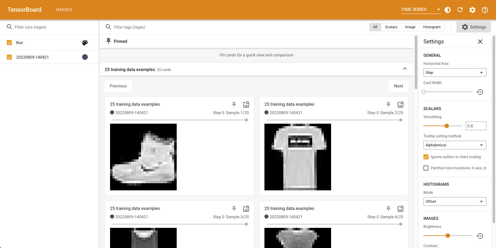
可视化多张图片

调整tf.summary.image里面的参数max_outputs：

 with file_writer.as_default():
    # Don't forget to reshape.
    images = np.reshape(train_images[0:25], (-1, 28, 28, 1))
    tf.summary.image("25 training data examples", images, max_outputs=25, step=0)

%tensorboard --logdir logs/train_data

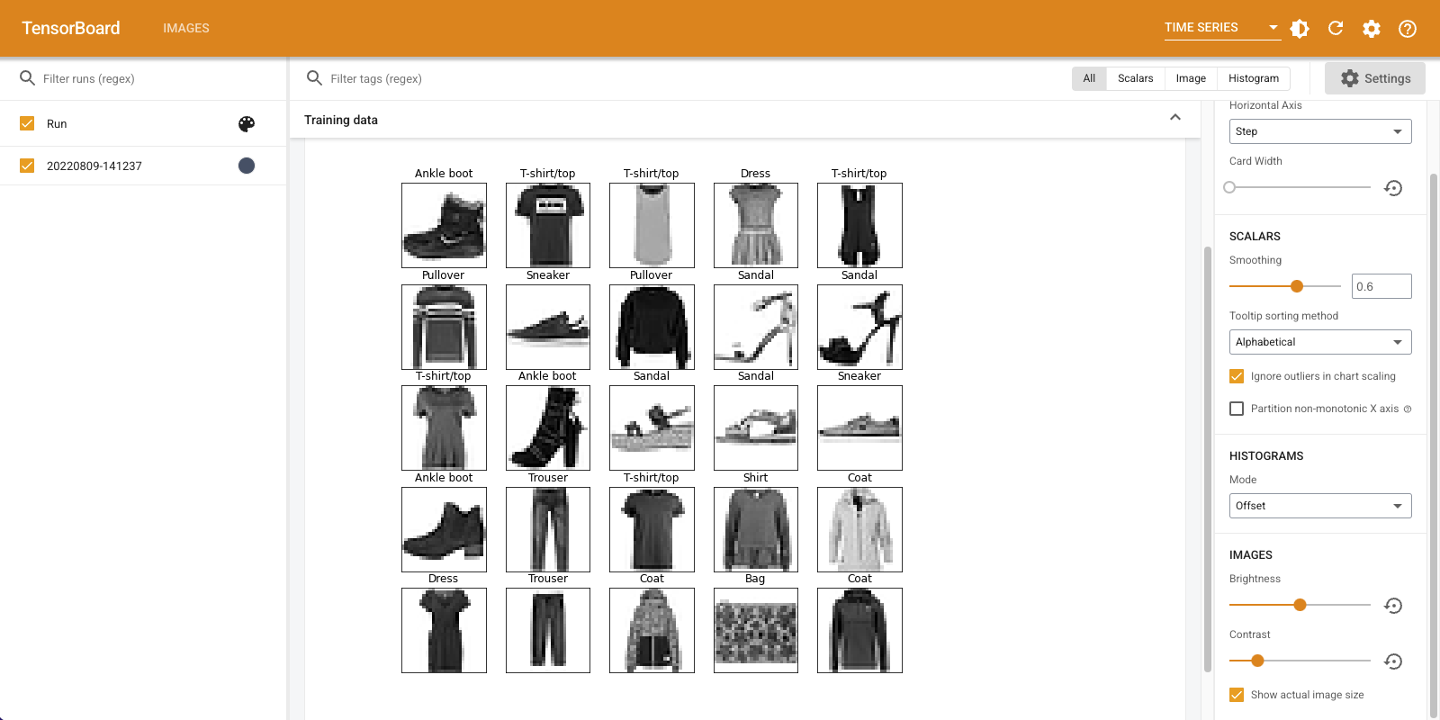
可视化其他格式的图片

有些图片不是tensor或者numpy.array，而是由诸如opencv、matplotlib生成的png图像，我们需要将其转化为tensor。

由于matplotlib适合生成复杂的数据图，因此先利用其他库生成图片，随后利用tf.summary.image将其转化为一个tensor再可视化，是一个比较方便的选择。

matplotlib生成数据集可视化：

 # Clear out prior logging data.
!rm -rf logs/plots

logdir = "logs/plots/" + datetime.now().strftime("%Y%m%d-%H%M%S")
file_writer = tf.summary.create_file_writer(logdir)

def plot_to_image(figure):
  """Converts the matplotlib plot specified by 'figure' to a PNG image and
  returns it. The supplied figure is closed and inaccessible after this call."""
  # Save the plot to a PNG in memory.
  buf = io.BytesIO()
  plt.savefig(buf, format='png')
  # Closing the figure prevents it from being displayed directly inside
  # the notebook.
  plt.close(figure)
  buf.seek(0)
  # Convert PNG buffer to TF image
  image = tf.image.decode_png(buf.getvalue(), channels=4)
  # Add the batch dimension
  image = tf.expand_dims(image, 0)
  return image

def image_grid():
  """Return a 5x5 grid of the MNIST images as a matplotlib figure."""
  # Create a figure to contain the plot.
  figure = plt.figure(figsize=(10,10))
  for i in range(25):
    # Start next subplot.
    plt.subplot(5, 5, i + 1, title=class_names[train_labels[i]])
    plt.xticks([])
    plt.yticks([])
    plt.grid(False)
    plt.imshow(train_images[i], cmap=plt.cm.binary)

  return figure

尔后，利用tf.summary.image转化：

# Prepare the plot
figure = image_grid()
# Convert to image and log
with file_writer.as_default():
  tf.summary.image("Training data", plot_to_image(figure), step=0)

最后，利用TensorBoard可视化：

%tensorboard --logdir logs/plots

在图片分类器中使用TensorBoard

之前我们通过TensorBoard了解了Fashion-MNIST数据集的概要，但是TensorBoard的功能不止于此。

首先构建分类模型：

model = keras.models.Sequential([
    keras.layers.Flatten(input_shape=(28, 28)),
    keras.layers.Dense(32, activation='relu'),
    keras.layers.Dense(10, activation='softmax')
])

model.compile(
    optimizer='adam', 
    loss='sparse_categorical_crossentropy',
    metrics=['accuracy']
)

我们想使用混淆矩阵详细了解分类器对测试数据的性能。因此接下来定义一个函数，专门计算混淆矩阵。具体来说，

1. 使用model.predict预测该epoch的所有测试用例的标签，得到test_pred
2. 调用sklearn.metrics.confusion_matrix直接计算混淆矩阵
3. 使用matplotlib将混淆矩阵可视化
4. 将matplotlib生成的图片转为tensor，最后变成log储存

下面是前两步所需的操作：

def log_confusion_matrix(epoch, logs):
    # Use the model to predict the values from the validation dataset.
    test_pred_raw = model.predict(test_images)
    test_pred = np.argmax(test_pred_raw, axis=1)

    # Calculate the confusion matrix.
    cm = sklearn.metrics.confusion_matrix(test_labels, test_pred)
    # Log the confusion matrix as an image summary.
    figure = plot_confusion_matrix(cm, class_names=class_names)
    cm_image = plot_to_image(figure)

    # Log the confusion matrix as an image summary.
    with file_writer_cm.as_default():
    tf.summary.image("Confusion Matrix", cm_image, step=epoch)

下面是第三步所需的可视化函数：

def plot_confusion_matrix(cm, class_names):
    """
    Returns a matplotlib figure containing the plotted confusion matrix.

    Args:
    cm (array, shape = [n, n]): a confusion matrix of integer classes
    class_names (array, shape = [n]): String names of the integer classes
    """
    figure = plt.figure(figsize=(8, 8))
    plt.imshow(cm, interpolation='nearest', cmap=plt.cm.Blues)
    plt.title("Confusion matrix")
    plt.colorbar()
    tick_marks = np.arange(len(class_names))
    plt.xticks(tick_marks, class_names, rotation=45)
    plt.yticks(tick_marks, class_names)

    # Normalize the confusion matrix.
    cm = np.around(cm.astype('float') / cm.sum(axis=1)[:, np.newaxis], decimals=2)

    # Use white text if squares are dark; otherwise black.
    threshold = cm.max() / 2.
    for i, j in itertools.product(range(cm.shape[0]), range(cm.shape[1])):
    color = "white" if cm[i, j] > threshold else "black"
    plt.text(j, i, cm[i, j], horizontalalignment="center", color=color)

    plt.tight_layout()
    plt.ylabel('True label')
    plt.xlabel('Predicted label')
    return figure

下面是第四步所需的tensor转化和储存函数以及其他回调函数：

# Clear out prior logging data.
!rm -rf logs/image

logdir = "logs/image/" + datetime.now().strftime("%Y%m%d-%H%M%S")
# Define the basic TensorBoard callback.
tensorboard_callback = keras.callbacks.TensorBoard(log_dir=logdir)
file_writer_cm = tf.summary.create_file_writer(logdir + '/cm')

让我们开始训练：

# Start TensorBoard.
%tensorboard --logdir logs/image

# Train the classifier.
model.fit(
    train_images,
    train_labels,
    epochs=5,
    verbose=0, # Suppress chatty output
    callbacks=[tensorboard_callback, cm_callback],
    validation_data=(test_images, test_labels),
)

请注意，此时我先调用的TensorBoard，然后开始的训练，并且我设置了verbose=0，意味着信息完全通过TensorBoard动态展示。训练过程中你就可以看到参数的变化。

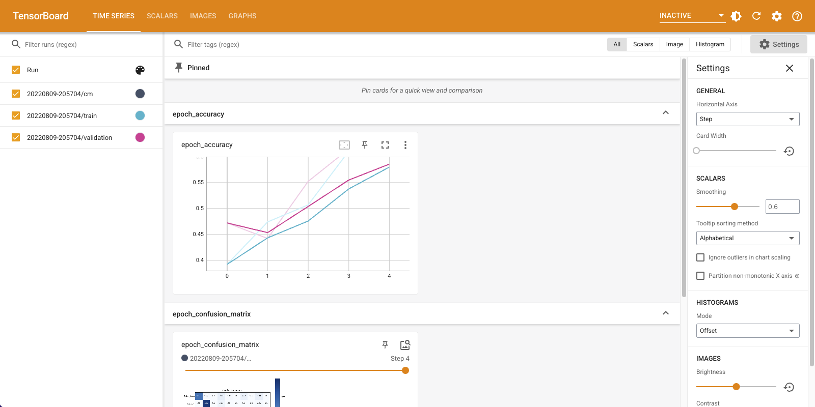
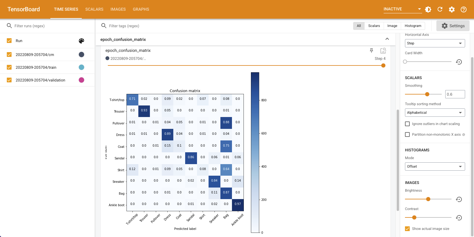
你还可以看到，随着训练的进行，矩阵是如何发生变化的：沿着对角线的正方形会逐渐变暗，而矩阵的其余部分趋向于0和白色。这意味着分类器正在不断改进。