总结词袋模型、Tf-idf等文本特征提取方法

一、词袋模型

文本数据通常被表示为由字符组成的字符串。我们需要先处理数据，然后才能对其应用机器学习算法。

在文本分析的语境中，数据集通常被称为语料库（corpus），每个由单个文本表示的数据点被称为文档（document）。

最简单的处理方法，是只计算语料库中每个单词在每个文本中的出现频次。这种文本处理模型称之为词袋模型。

不考虑词语出现的顺序，每个出现过的词汇单独作为一列特征，这些不重复的特征词汇集合为词表。

每一个文本都可以在很长的词表上统计出一个很多列的特征向量。如果每个文本都出现的词汇，一般被标记为停用词不计入特征向量。

为了搞清楚词袋模型，也就是CountVectorizer到底做了什么，我们执行以下代码：

bards_words =["The fool doth think he is wise,",
    "but the wise man knows himself to be a fool"]

我们导入 CountVectorizer 并将其实例化，然后对 bards_words 进行拟合，如下所示：

from sklearn.feature_extraction.text import CountVectorizer
vect = CountVectorizer()
vect.fit(bards_words)

拟合 CountVectorizer 包括训练数据的分词与词表的构建，我们可以通过 vocabulary_ 属性来访问词表：

print("Vocabulary size: {}".format(len(vect.vocabulary_)))
print("Vocabulary content:\n {}".format(vect.vocabulary_))
#------------------#
Vocabulary size: 13
Vocabulary content:
{'the': 9, 'himself': 5, 'wise': 12, 'he': 4, 'doth': 2,
 'to': 11, 'knows': 7,'man': 8, 'fool': 3, 'is': 6, 'be': 0, 
 'think': 10, 'but': 1}

词表共包含 13 个词，从 “be” 到 “wise”。
我们可以调用 transform 方法来创建训练数据的词袋表示：

bag_of_words = vect.transform(bards_words)
print("bag_of_words: {}".format(repr(bag_of_words)))
#--------------------#
bag_of_words: <2x13 sparse matrix of type '<class 'numpy.int64'>'
with 16 stored elements in Compressed Sparse Row format>

词袋表示保存在一个 SciPy 稀疏矩阵中，这种数据格式只保存非零元素。这个矩阵的形状为 2×13，每行对应于两个数据点之一，每个特征对应于词表中的一个单词。要想查看稀疏矩阵的实际内容，可以使用 toarray 方法将其转换为“密集的”NumPy 数组（保存所有 0 元素）：

print("Dense representation of bag_of_words:\n{}".format(
    bag_of_words.toarray()))
#---------------------#
Dense representation of bag_of_words:
[[0 0 1 1 1 0 1 0 0 1 1 0 1]
[1 1 0 1 0 1 0 1 1 1 0 1 1]]

删除没有信息量的单词，除了使用min_df参数设定词例至少需要在多少个文档中出现过之外，还可以通过添加停用词的方法。

二、用tf-idf缩放数据

词频 - 逆向文档频率（term frequency–inverse document frequency，tf-idf）方法，对在某个特定文档中经常出现的术语给予很高的权重，但对在语料库的许多文档中都经常出现的术语给予的权重却不高。

scikit-learn 在两个类中实现了 tf-idf 方法：TfidfTransformer 和 TfidfVectorizer，前者接受 CountVectorizer 生成的稀疏矩阵并将其变换，后者接受文本数据并完成词袋特征提取与 tf-idf 变换。

单词w在文档d中的tf-idf分数为：

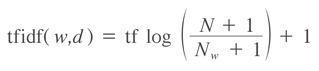
式中，tf为词频，Term Frequency, 表示一个词在一个文档中的出现频率。该频率最后要除以该文档的长度，用以归一化。

式中，$N$为总文档数，$N_w$为带有单词$w$的文档数。由于分子比分母大，所以该 $\log$ 值必不可能小于零。

from sklearn.feature_extraction.text import TfidfVectorizer
corpus=["I come to China to travel",
"This is a car polupar in China",
"I love tea and Apple ",
"The work is to write some papers in science"]
tfidf = TfidfVectorizer()
vector = tfidf.fit_transform(corpus)
print(vector)

#---------------#
(0, 16)    0.4424621378947393
(0, 3)    0.348842231691988
(0, 15)    0.697684463383976
(0, 4)    0.4424621378947393
(1, 5)    0.3574550433419527
(1, 9)    0.45338639737285463
(1, 2)    0.45338639737285463
(1, 6)    0.3574550433419527
(1, 14)    0.45338639737285463
(1, 3)    0.3574550433419527
(2, 1)    0.5
(2, 0)    0.5
(2, 12)    0.5
(2, 7)    0.5
(3, 10)    0.3565798233381452
(3, 8)    0.3565798233381452
(3, 11)    0.3565798233381452
(3, 18)    0.3565798233381452
(3, 17)    0.3565798233381452
(3, 13)    0.3565798233381452
(3, 5)    0.2811316284405006
(3, 6)    0.2811316284405006
(3, 15)    0.2811316284405006

返回值什么意思呢？(0, 16)代表第0个文档，第一个单词在单词表（词袋）中的位置是第16个，该单词的tf-idf值为0.44246213；第二个单词在词袋中第3个位置……

显然这是个经过压缩的系数矩阵，每一行的元组表明该元素在稀疏矩阵中的位置，其值为右边的tf-idf值，代表一个单词。可以通过.toarray()方法令其恢复到系数矩阵状态。

print(vector.toarray().shape)
print(len(vector.toarray()))
print(type(vector.toarray()))
print(vector.toarray())
#-----------------------------#
(4, 19)
4
<class 'numpy.ndarray'>
[[0. 0. 0. 0.34884223 0.44246214 0.
  0. 0. 0. 0. 0. 0.
  0. 0. 0. 0.69768446 0.44246214 0.
  0. ]

 [0. 0. 0.4533864  0.35745504 0. 0.35745504
  0.35745504 0. 0. 0.4533864  0. 0.
  0. 0. 0.4533864  0. 0. 0.
  0. ]

 [0.5 0.5 0. 0. 0. 0.
  0. 0.5 0. 0. 0. 0.
  0.5 0. 0. 0. 0. 0.
  0. ]

 [0. 0. 0. 0. 0. 0.28113163
  0.28113163 0. 0.35657982 0. 0.35657982 0.35657982
  0. 0.35657982 0. 0.28113163 0. 0.35657982
  0.35657982]]

三、多元词袋

词袋模型将一段文档拆分成单词后，忽略了单词的上下文可能对文档的含义造成影响。

四、英语的词干提取与词形还原

五、中文的分词

六、主题建模与文档聚类